Quickstart
Making a lightcurve — This is likely the basic task that you need SPIDERMAN to perform, to, for example, form the basis for a likelihood function being fed into an mcmc. Here is how to return a simulated lightcurve from SPIDERMAN, the fast way.
First, import spiderman into the namespace:
import spiderman as sp
Now, it is necesarry to generate a parameter object, this will be the main way of interacting with the code. Before doing so, you must specify which brightness model (link to brightness model page) you wish to use. In this example we will use the analytical formula from Zhang & Showman 2016, but many other options are availible (If you have a brightness model that is not represented, please contact me, and I will include it in the next release of the package).
spider_params = sp.ModelParams(brightness_model="zhang")
Now that the parameter object has been created, we can define the parameters as so:
spider_params.n_layers= 5
This parameter refers to the number of layers in the 2d “web” used to define the integration grid. 5 is typically acceptable for most availible data qualities. Next we will define the system parameters, using values suitable for WASP-43b
spider_params.t0= 200               # Central time of PRIMARY transit [days]
spider_params.per= 0.81347753       # Period [days]
spider_params.a_abs= 0.01526        # The absolute value of the semi-major axis [AU]
spider_params.inc= 82.33            # Inclination [degrees]
spider_params.ecc= 0.0              # Eccentricity
spider_params.w= 90                 # Argument of periastron
spider_params.rp= 0.1594            # Planet to star radius ratio
spider_params.a= 4.855              # Semi-major axis scaled by stellar radius
spider_params.p_u1= 0               # Planetary limb darkening parameter
spider_params.p_u2= 0               # Planetary limb darkening parameter
Note
these definitions are compatible with Batman (Kreidberg et al 2015)
Now set the parameters specific to the brightness model that we defined earlier:
spider_params.xi= 0.3       # Ratio of radiative to advective timescale
spider_params.T_n= 1128     # Temperature of nightside
spider_params.delta_T= 942  # Day-night temperature contrast
spider_params.T_s = 4500    # Temperature of the star
Since this uses model spectra, it is necessary to specify the bandpass with these parameters:
spider_params.l1 = 1.1e-6       # The starting wavelength in meters
spider_params.l2 = 1.7e-6       # The ending wavelength in meters
Warning
SPIDERMAN calculates ratios in flux density assuming a response function that is uniform in energy flux. If you want a response uniform in photon counts you must define a instrument response function (see Instrument Response section).
Now, define the times you wish the model to be evaluated at, let’s do a single full orbit:
t= spider_params.t0 + np.linspace(0, + spider_params.per,100)
Finally, a lightcurve can be generated simply by using the “lightcurve” method:
lc = spider_params.lightcurve(t)
plt.plot(t,lc)
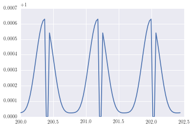
The resulting lightcurve
Warning
SPIDERMAN currently only produces secondary eclipses and phase-curves - the primary eclipse will not be modelled! To model the primary eclipse an additional code, such as BATMAN (Kreidberg et al 2015) will be required.
It’s that simple!